|
STA
6166 UNIT 3 Section 3 Answers
|
| Welcome | < | Begin | < | < | Unit 3 Section 3 Answers | |||||
| To Ag and Env. Answers |
| To Tox and Health Answers |
| To Social and Education Answers |
| To Engineering Answers |
Unit 3 Section 3 Answers
Social and Education
1. A company uses a pre-employment test to screen applicants for sales jobs.
We are interested in whether the screning test is effective. In an experiment,
a random samples of applicants who pass the test
and a second sample of those who do not pass the screening test are all employed.
The number of employees who successfully completed the training program in
these two samples was recorded as follows.
| Experiment Result |
Applicant who pass the pre-employment
test
|
Applicant who do not pass the pre-employment
test
|
| Employees completed in the training
program |
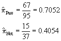
67
|
15
|
| Employees failed in the training
program |
28
|
22
|
| Total number of Employees |
95
|
37
|
a. Test whether the proportions of employee who successfully completed the training program is the same for the group who initially passed the pre-employment test to those who did not initially pass the pre-emplyment test. For this test use P(Type I error)=a=.05.
H0: pPass - pNot = 0
HA: pPass - pNot not equal to 0
T.S.: 
RR: Reject if |z| > za/2=z0.025 = 1.96
Here, the test statistic value is 3.203 which is greater than 1.96 causing us to reject the null hypothesis and conclude that there is a significant difference between the completion rates for applicants who successfully pass the pre-employment test and those who do not. Clearly, the pre-employment test has some ability to screen applicants and increase completion rates for subsequent training.
b. Calculate a 95% confidence interval for the above difference.
The 95% confidence interval is computed using the equation:
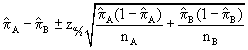
[0.2988 ± 1.96(0.09329)] or [0.2988 ± 0.1828] or [0.1159, 0.48165]
Note that the 95% CI does not contain zero, a good indication that the difference is not statistically equal to zero.
|
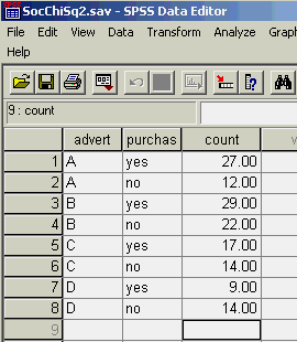
Four
types of advertisement |
Customers
made purchases |
Total
|
|
1.Advertisement
A |
27 |
39 |
|
2.Advertisement
B |
29 |
51 |
|
3.Advertisement
C |
17 |
31 |
|
4
Advertisement D |
9 |
23 |
Can we determine from this whether there is a difference in the purchase fraction across the four groups?
These data represent a 2 by 4 contingency table but is presented in odd format. More commonly you would expect to see a table like the one below.
|
Purchase
|
|||
|
Yes
|
No
|
||
| Advertisement |
A
|
27
|
12
|
|
B
|
29
|
22
|
|
|
C
|
17
|
14
|
|
|
D
|
9
|
14
|
|
We will use SPSS to analyse these data. We create the following dataset.
The Chi Square analysis is part of the ANALYZE > DESCRIPTIVE STATISTICS > CROSSTABS options, but first we have to tell SPSS that the frequency counts for the advertisement by purchase combinations is in the count column. This is done with the DATA > WEIGHT CASES option. In the resulting dialog we set Weight Case By [COUNT]. Once this is done, we are ready to specify options in the ANALYZE > DESCRIPTIVE STATISTICS > CROSSTABS dialog box. Set Rows to Advent, Cols to Purchuse, Statistics to Chi Square, and in the Cells dialog check Observed, Expected, Row, Column, Total. The resulting output follows.
| PURCHASE | Total | ||||
|---|---|---|---|---|---|
| no | yes | ||||
| ADVERT | A | Count | 12 | 27 | 39 |
| Expected Count | 16.8 | 22.2 | 39.0 | ||
| % within ADVERT | 30.8% | 69.2% | 100.0% | ||
| % within PURCHASE | 19.4% | 32.9% | 27.1% | ||
| % of Total | 8.3% | 18.8% | 27.1% | ||
| B | Count | 22 | 29 | 51 | |
| Expected Count | 22.0 | 29.0 | 51.0 | ||
| % within ADVERT | 43.1% | 56.9% | 100.0% | ||
| % within PURCHASE | 35.5% | 35.4% | 35.4% | ||
| % of Total | 15.3% | 20.1% | 35.4% | ||
| C | Count | 14 | 17 | 31 | |
| Expected Count | 13.3 | 17.7 | 31.0 | ||
| % within ADVERT | 45.2% | 54.8% | 100.0% | ||
| % within PURCHASE | 22.6% | 20.7% | 21.5% | ||
| % of Total | 9.7% | 11.8% | 21.5% | ||
| D | Count | 14 | 9 | 23 | |
| Expected Count | 9.9 | 13.1 | 23.0 | ||
| % within ADVERT | 60.9% | 39.1% | 100.0% | ||
| % within PURCHASE | 22.6% | 11.0% | 16.0% | ||
| % of Total | 9.7% | 6.3% | 16.0% | ||
| Total | Count | 62 | 82 | 144 | |
| Expected Count | 62.0 | 82.0 | 144.0 | ||
| % within ADVERT | 43.1% | 56.9% | 100.0% | ||
| % within PURCHASE | 100.0% | 100.0% | 100.0% | ||
| % of Total | 43.1% | 56.9% | 100.0% | ||
| Value | df | Asymp. Sig. (2-sided) | |
|---|---|---|---|
| Pearson Chi-Square | 5.434(a) | 3 | .143 |
| Likelihood Ratio | 5.484 | 3 | .140 |
| N of Valid Cases | 144 | ||
| a 0 cells (.0%) have expected count less than 5. The minimum expected count is 9.90. | |||
The Chi Square statistic computed for this table is 5.434 with associated p-value of 0.143. This is larger than the 0.05 Type I error rate we chose to use initially hence we would NOT reject the null hypothesis of independence between advertisement and purchase decision. This suggests that the decision to purchase does not seem to depend on any particular advertisement, although, the difference between observed and expected counts in the D advertisement is the largest observed in the table.