|
STA
6166 UNIT 3 Section 1 Answers
|
| Welcome | < | Begin | < | < | Unit 3 Section 1 Answers | > | Section 2 | |||||
| To Ag and Env. Answers |
| To Tox and Health Answers |
| To Social and Education Answers |
| To Engineering Answers |
Unit 3 Section 1 Answers
Toxicology and Health
From problem 9.24,page 464 in Ott and Longnecker. Researchers conducted a study of the effects of three heartworm drugs on the fat content of the shoulder muscles in Labrador retrievers. Twenty (20) dogs were randomly divided into four treatment groups of five (5) dogs each. Dogs in group A were assigned to the untreated control. The remaining three groups identify which of the heartworm drug all dogs in the group received. At the end of two years of treatment, the percentage fat content of the shoulder muscles was determined and is given here.
 A    B    C    D
2.64 3.24 2.90 2.91
2.56 3.71 3.02 2.89
3.30 2.95 3.78 3.21
2.19 3.01 2.96 2.89
2.45 3.08 2.87 2.68
- Write the linear model for these data.
- Perform a one-way analysis of variance. Test the hypothesis of no differences in average fat content at a type I error rate of 5%.
- Test the hypothesis of equal variances. Do these data need to be transformed? If so, what transformation would you use?
- For each group, compute the sample mean and subtract this mean from each observation (i.e. center each group's data). Combine all these "residuals" into on data set and test for normality. Is there any indication that these data are not normal.
- Perform the Kruskal-Wallis test on these data. How do the results compare to the analysis of variance procedure?
Answers:
1. yij = m + ai + eij
-
yij - the fat content of the j-th dog from the i-th treatment group(1=A, 2=B, 3=C, 4=D).
-
m - the overall mean fat content (if all dogs had the same treatment, its average fat content would be this.)
- ai - the (average) effect of the i-th treatment on overall average fat content- how much the i-th treatment changes the average dog's fat contentr from the overall mean, m.
- eij - the residual left over once we remove the overall mean and the effect of the i-th treatment from the (ij)-th observation - assumed to have common variance estimated by the MSE and zero mean.
2. This problem has analysis that follows closely that described in the Engineering example. Look at that problem for a detailed writeup. The SAS program for this analysis can be found here. The full output can be found here. Here I will only provide the final tables and graphs.
Dependent Variable: fat
                                      Sum of
Source                     DF        Squares    Mean Square   F Value   Pr > F
Model                       3     0.95052000     0.31684000      2.85   0.0703
Error                      16     1.77920000     0.11120000
Corrected Total            19     2.72972000

Level of            -------------fat-------------
treatment     N             Mean          Std Dev
A             5       2.62800000       0.41227418
B             5       3.19800000       0.30605555
C             5       3.10600000       0.38115614
D             5       2.91600000       0.18942017

Bartlett's Test for Homogeneity of fat Variance
Source           DF    Chi-Square    Pr > ChiSq
treatment         3        2.2137        0.5293

   Brown and Forsythe's Test for Homogeneity of fat Variance
        ANOVA of Absolute Deviations from Group Medians

                         Sum of        Mean
Source           DF     Squares      Square    F Value    Pr > F
treatment         3      0.0579      0.0193       0.26    0.8513
Error            16      1.1752      0.0734

                   Tests for Normality

Test                  --Statistic---    -----p Value-----
Shapiro-Wilk          W     0.840287    Pr < W      0.004
Kolmogorov-Smirnov    D     0.245416    Pr > D     <0.010
Cramer-von Mises      W-Sq  0.240502    Pr > W-Sq  <0.005
Anderson-Darling      A-Sq  1.351514    Pr > A-Sq  <0.005

Kruskal-Wallis one way analysis of variance
 for 2-year dog fat data for Problem 9.24

The NPAR1WAY Procedure

              Wilcoxon Scores (Rank Sums) for Variable fat
                    Classified by Variable treatment

                         Sum of      Expected       Std Dev          Mean
treatment       N        Scores      Under H0      Under H0         Score
--------------------------------------------------------------------------
A               5          28.0         52.50     11.452131          5.60
B               5          75.0         52.50     11.452131         15.00
C               5          61.0         52.50     11.452131         12.20
D               5          46.0         52.50     11.452131          9.20

                   Average scores were used for ties.


   Kruskal-Wallis Test
Chi-Square         6.9824
DF                      3
Pr > Chi-Square    0.0725
Figure 1. Histogram of residuals with overlay of normal density curve.
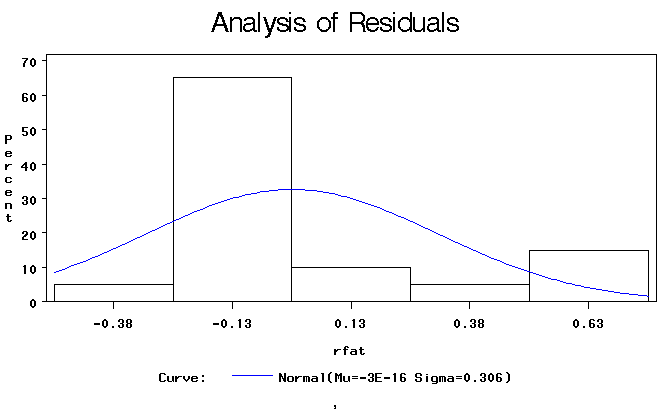
Figure 2. Normal probability plot of residuals.
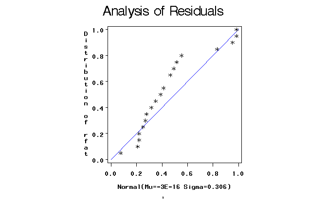
The formal normality test and the probability plot suggest that possibly these data could benifit from a transformation. But what transformation? Plotting the treatment sample means versus the sample variances or even standard deviations suggests that none of the standard transformation would work.
Figure 3. Plot of treatment sample means versus variances.
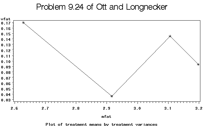
Since the tests of variances do not reject the null hypothesis of equal variances and there seems no obvious way to transform the data that would simultaneously maintain homogeneity while providing for more normally distributed residuals, we will tentatively accept the analysis of variance on the untransformed observations and conclude that there are no treatment differences (p-value = 0.07 which is greater than our a=0.05 typical test level.)
We compute the non-parameteric Kruskal-Wallis test statistics as a further check on our decision. The results of the test suggest further that there are no statistically significant differences among the treatments (p-value = 0.0725).