|
STA
6166 UNIT 3 Section 1 Answers
|
| Welcome | < | Begin | < | < | Unit 3 Section 1 Answers | > | Section 2 | |||||
| To Ag and Env. Answers |
| To Tox and Health Answers |
| To Social and Education Answers |
| To Engineering Answers |
Unit 3 Section 1 Answers
Engineering
Problem 8.30, page 424 of Ott and Longnecker. A small corporation make insulation shields for electrical wires using three different types of machines. The corporation wants to evaluate the variation in the inside diameter dimension of the shields produced by the machines. A quality engineer at the corporation randomly selects shields produced by each of the machines and records the inside diameters of each shield (in millimeters). She wants to determine whether the means and standard deviations of the three machines differ. The data are given below.
Machine_C  Machine_B  Machine_A
 29.7        8.7         18.1
 18.7       56.8          2.4
 16.5        4.4          2.7
 63.7        8.3          7.5
 18.9        5.8         11.0
107.2         .            .
 19.7         .            .
 93.4         .            .
 21.6         .            .
 17.8         .            .
- Write the linear model for these data.
- Perform a one-way analysis of variance. Test the hypothesis of no differences in average shield diameters at a type I error rate of 5%.
- Test the hypothesis of equal variances. Do these data need to be transformed? If so, what transformation would you use?
- For each machine, compute the sample mean and subtract this mean from each observation (i.e. center each machine's data). Combine all these "residuals" into on data set and test for normality. Is there any indication that these data are not normal.
- Perform the Kruskal-Wallis test on these data. How do the results compare to the analysis of variance procedure?
Answers:
yij = m + ai + eij
-
yij - the diameter of the j-th shield from the i-th machine (1=A, 2=B, 3=C).
-
m - the overall mean diameter (if all shields were run on the same machine its average diameter would be this.)
- ai - the (average) effect of the i-th machine on overall yield- how much the i-th machnie changes the average shield diameter from the overall mean, m.
- eij - the residual left over once we remove the overall mean and the effect of the i-th machnie from the (ij)-th observation - assumed to have common variance estimated by the MSE and zero mean.
2. We will use SAS Proc GLM to obtain the computations of the AOV. The SAS program is fairly long and can be found here. This program has comments describing what the purpose is of each procedure. Use the SAS help files to understand what each procedure does. The full output from the SAS program can be viewed here. Note that SAS can produce a lot of output. The AOV table is reproduced below. Note that with a p-value (Pr>F)=0.0939 we would not reject the null hypothesis of equal machine means at the a=0.05 level.
Table 1. Analysis of variance table for the test of the hypothesis of equal machine means.
                                      Sum of
Source                     DF        Squares    Mean Square   F Value   Pr > F
Model                       2     4141.04150     2070.52075      2.73   0.0939
Error                      17    12907.38800      759.25812
Corrected Total            19    17048.42950
The Means statement in the Proc GLM block has the option to perform tests for homogeneity of variances. Here I have asked it to consider two tests, Bartlett's and Brown and Forsythe' s modification of Levene's test. The results are reproduced here.
Table 2. Machine means and standard deviations with associated test statistics of the hypothesis of equal machine variances.
Level of            -----------diameter----------
machine       N             Mean          Std Dev
a             5        8.3400000        6.5217329
b             5       16.8000000       22.4311168
c            10       40.7200000       34.5199395

Bartlett's Test for Homogeneity of diameter Variance

Source         DF    Chi-Square    Pr > ChiSq
machine         2        8.3489        0.0154

Brown and Forsythe's Test for Homogeneity of diameter Variance
       ANOVA of Absolute Deviations from Group Medians

                       Sum of        Mean
Source         DF     Squares      Square    F Value    Pr > F
machine         2      1144.9       572.4       0.84    0.4480
Error          17     11555.8       679.8
Bartlett's test suggests there are significant heterogeneity of variances whereas the BF test suggest the variances are the same. Note in the table the large differences between the machine A standard deviation and the machine C standard deviation. Despite the BF tests results, I might be a little uneasy about the assumption of common variance. But we reserve judgement until we look at the normality of residuals.
The statistics for testing the normality of residuals are computed in Proc Capability. The important part of this analysis is given below.
Table 3. Test statistics for assessing normality of residuals from the analyis of variance model.
                   Tests for Normality
Test                  --Statistic---    -----p Value-----
Shapiro-Wilk          W     0.811160    Pr < W      0.001
Kolmogorov-Smirnov    D     0.235658    Pr > D     <0.010
Cramer-von Mises      W-Sq  0.255007    Pr > W-Sq  <0.005
Anderson-Darling      A-Sq  1.438729    Pr > A-Sq  <0.005
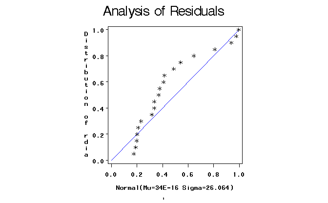
Note that the Shapiro-Wilk test (and all othere tests we have not covered in this class) suggest that the residuals are not normally distributed. Histograms and normal probability plots of the residuals back up these tests.
Figure 1. Histogram of residuals with overlay of normal density curve.

Figure 2. Normal Probability Plot of residuals.

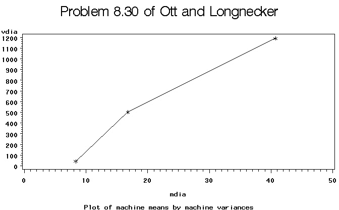
Note that the residuals do not look very normal. To determine what form of transformation might be used, we plot the machine sample means versus the machine sample variances and look for linearity.
Figure 3. Plot of sample means and variances for the three machines.

The relationship is fairly linear suggesting that a square root transformation should be used. Rerunning the analysis on the square root transformed data suggests that there are significant differences between machines in the average diameters when measured on the square root scale.
Table 4. Test statistics for square root transformed diameters.
Dependent Variable: sdia
                                      Sum of
Source                     DF        Squares    Mean Square   F Value   Pr > F
Model                       2     41.4272950     20.7136475      4.48   0.0274
Error                      17     78.6683337      4.6275490
Corrected Total            19    120.0956287

Level of            -------------sdia------------
machine       N             Mean          Std Dev
a             5       2.70040161       1.14446010
b             5       3.57461248       2.24224933
c            10       5.94879442       2.43398279

Bartlett's Test for Homogeneity of sdia Variance
Source         DF    Chi-Square    Pr > ChiSq
machine         2        2.2835        0.3193

  Brown and Forsythe's Test for Homogeneity of sdia Variance
       ANOVA of Absolute Deviations from Group Medians
                       Sum of        Mean
Source         DF     Squares      Square    F Value    Pr > F
machine         2      2.2704      1.1352       0.31    0.7364
Error          17     61.9489      3.6441

                   Tests for Normality
Test                  --Statistic---    -----p Value-----
Shapiro-Wilk          W     0.801182    Pr < W      0.001
Kolmogorov-Smirnov    D     0.246866    Pr > D     <0.010
Cramer-von Mises      W-Sq  0.278129    Pr > W-Sq  <0.005
Anderson-Darling      A-Sq  1.593010    Pr > A-Sq  <0.005
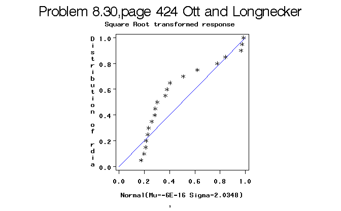
The tests of normality of residuals again suggest that residuals are not truely normal, but the Homogeneity of Variance tests suggest much stronger similarity in variances across machines.
Figure 4. Normal probability plot of residuals from the analysis of variance on square root transformed diameters.

There is no guarantee that any other transformation will do any better than the square root transformation. At this point we might consider performing a non-parameteric analysis of variance test to confirm or deny the existance of Machine differences in mean diameter. Since the non-parameteric test depends on ranks and not the original values, and the square root transformation does not change the ranks, we simply perform the analysis on the original data.
The non-parameteric test of choice here is the Kruakal-Wallis procedure. Results of this analysis are in the SAS output. The important parts of this analysis are presented below.
Table 5 Test statistics associated with the Kurskal-Wallis procedure.
Kruskal-Wallis one way analysis of variance
 for diameter data for Problem 8.30

The NPAR1WAY Procedure
           Wilcoxon Scores (Rank Sums) for Variable diameter
                    Classified by Variable machine

                       Sum of      Expected       Std Dev          Mean
machine       N        Scores      Under H0      Under H0         Score
------------------------------------------------------------------------------------------------------------------
a             5          27.0         52.50     11.456439          5.40
b             5          37.0         52.50     11.456439          7.40
c            10         146.0        105.00     13.228757         14.60

   Kruskal-Wallis Test
Chi-Square         9.8914
DF                      2
Pr > Chi-Square    0.0071
The p-value for the KW test (Pr > Chi-Square)=0.0071
suggests that we should reject the null hypothesis of equal machine MEDIANS
and entertain the alternative hypothesis of unequal median responses. Note that
the results of the Kruskal-Wallis test are similar to that obtained with the
analysis on the square root transformed responses and is different from that
observed with the untransformed diameters. The importance of satisfying the
homogeneity of variance and normality of residuals assumptions is illustrated
in this example.