|
STA
6166 UNIT 3 Section 1 Answers
|
| Welcome | < | Begin | < | < | Unit 3 Section 1 Answers | > | Section 2 | |||||
| To Ag and Env. Answers |
| To Tox and Health Answers |
| To Social and Education Answers |
| To Engineering Answers |
Unit 3 Section 1 Answers
Social and Education
A large advertising firm specializes in creating television commercials for children's products. A study is designed to test whether there are large differences in attention span for children in three different age groups (Group A 5-6 years, Group B 7-8 years, Group C 9-10 years). Ten children for each group are selected at random from a large population of children and asked to watch a 60-second breakfast cereal commercial. Researchers record their attention span during the viewing of the commercial. Times (in seconds) are given below.
 A  B  C
19 19 37
36 35  6
40 22 28
30 28  4
 4  1 32
10 27 16
30 27  8
 5 16 41
34  3 29
21 18 18
- Write the linear model for these data.
- Perform a one-way analysis of variance. Test the hypothesis of no differences in average attention time at a type I error rate of 5%.
- Test the hypothesis of equal variances. Do these data need to be transformed? If so, what transformation would you use?
- For each group, compute the sample mean and subtract this mean from each observation (i.e. center each group's data). Combine all these "residuals" into on data set and test for normality. Is there any indication that these data are not normal.
- Perform the Kruskal-Wallis test on these data. How do the results compare to the analysis of variance procedure.
Answers:
1. yij = m + ai + eij
-
yij - the attention span of the j-th child from the i-th age group(1=A, 2=B, 3=C, 4=D).
-
m - the overall mean attention span (if all children were from the same age group, its average attention span would be this.)
- ai - the (average) effect of the i-th age group on overall average attention span- how much the i-th age group changes the average child's attention span from the overall mean, m.
- eij - the residual left over once we remove the overall mean and the effect of the i-th age group from the (ij)-th observation - assumed to have common variance estimated by the MSE and zero mean.
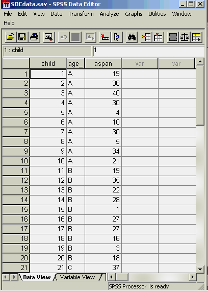
We will use SPSS to compute the statistics needed to answer questions 2-5 above. First we need to input the data into SPSS. If will be best if the data are in "stacked" form instead of the "unstacked" structure presented in the problem definition above. To get the data into stacked form, we cut from above and copy into EXCEL. Then in EXCEL we use cut and paste to get the attention span data stacked one column on top of the other. We add columns for child ID and age class, resulting in the following structure for the data in SPSS (not all the data are in view - you can download the SPSS sav file for this from here to see the whole dataset.).

The analysis of variance table and other associated statistics can be obtained using the following sequence of commands:
Analyse > General Linear Model > Univariate [Dependent Variable (aspan), Fixed Factor(s): Age_Group] > Save [Residuals - check unstandardized] > Continue > Options [Display Means for: age _grou, check Homogeneity tests and Descriptive statistics]> Continue > OK.
This produces a series of output tables which are produced below.

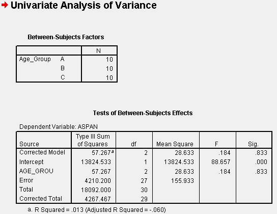
This provides us with the overall analysis of variance table. Of interest to us is the row labeled "AGE_GROU". The associated F-statistic (88.657) with 2 and 27 degrees of freedom tests the null hypothesis of equal average attention spans for each age group. In this case, the associated p-value is 0.833, leading us to NOT reject the null hypothesis of equal average attention spans at the a=0.05 Type I error rate. But before we fully accept this decision, we need to check out the assumptions for the analysis of variance.
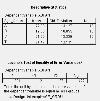
Levene's test for equality of error variances results from the Options > Homogeneity test selection we made from the original General Linear Models dialog.

From the above, we have a p-value associated with the test of equal variances of 0.422, suggesting that we should NOT reject the null hypothesis of equal variances. From the table of descriptive statistics we see that the standard deviations are not particularly different.
The residuals were stored in the res_1 column in the worksheet. The Kolmogorov-Smirinov and Shipiro-Wilk tests are readily available in SPSS from the following request:
Analyse > Descriptive statistics > Explore [Dependent list: residuals for aspan] > Plots [check normality plots with tests].

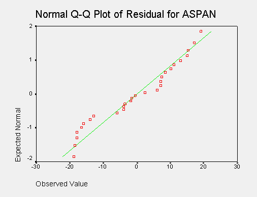
This suggests that the residuals may not be normally distributed, but the normal probability plot of the residuals below shows that the data that is not very non-normal. Since the F test in the analysis of variance is not very sensitive to non-normnality we choose to not pursue further analysis via transformations.

To double check our decision, we choose to run the non-parametric Kruskal-Wallis test procedure on the data. In SPSS this is accomplished by the following commands:
Analyse > Nonparametric tests> K Independent samples.
Note that when we try to run this test with our existing dataset, we cannot see our grouping factor, Age_Group in the list of variables. This must be an oddity of SPSS in that it requires numeric grouping codes for nonparametric tests. To create this numeric code, use the SPSS Data Window commands: Transform > Recode > Into different variables [Input variable: Age_Grou; Output variable: Group] > Old and New Values > Check first "Convert numeric strings to numbers", then Old Value: A; New Value: 1; Add; Old Value: B; New Value: 2; Add; Old Value: C; New Value: 3; Add; Old Value: C; New Value: 4; Add]>Continue > Change > OK. Now you have a new variable on your datasheet called Group which has numbers for the age group codes instead of letters. Returning to the Analyse > Nonparametric tests> K Independent samples dialog, now we do: Test Variable List: aspan; Grouping Variable List: Group > Define Range [minimum: 1, maximum: 4] > Continue > OK.

The p-value associated with the null hypothesis of equal group medians is reported to be 0.627 leading us to NOT reject the null hypothesis of equal group medians. This test supports the conclusion of the regular analysis of variance.