Unit 3 Section 1 Answers

Ag and Environment

Problem 8.17 in Ott and Longnecker. Researchers record the yields of corn, in bushels per plot, for four different varieties of corn, A, B, C, and D. In a controlled greenhouse experiment, the researchers randomly assign each variety to eight of 32 plots available for the study. The yields are listed here.

 A   B   C   D
2.5 3.6 4.3 2.8
3.6 3.9 4.4 2.9
2.8 4.1 4.5 3.1
2.7 4.3 4.1 2.4
3.1 2.9 3.5 3.2
3.4 3.5 3.4 2.5
2.9 3.8 3.2 3.6
3.5 3.7 4.6 2.7

1. Write the linear model for these data.

y_ij = m + a_i + e_ij

y_ij - the yield of the j-th plot from the i-th variety (1=A, 2=B, 3=C, 4=D).
m - the overall mean yield (if all plots had the same treatment its average yield would be this.)
a_i - the (average) effect of the i-th variety on overall yield- how much the i-th variety changes the average yield from the overall mean, m.
e_ij - the residual left over once we remove the overall mean and the effect of the i-th variety from the (ij)-th observation - assumed to have common variance estimated by the MSE and zero mean.

2. Perform a one-way analysis of variance. Test the hypothesis of no differences in average yields at a type I error rate of 5%.

3. Test the hypothesis of equal variances. Do these data need to be transformed? If so, what transformation would you use?

4. For each variety, compute the sample mean and subtract this mean from each observation (i.e. center each variety). Combine all these "residuals" into on data set and test for normality. Is there any indication that these data are not normal.

5.Perform the Kruskal-Wallis test on these data. How do the results compare to the analysis of variance procedure

We will use Minitab to solve this problem. The data should be stacked to run all of the above analyses. In addition we will use both numberic codes and alphabetic codes for the variaty names. Below is a partial printout of the worksheet (wouldn't all fit on the screen for a screen capture.)

The analysis of variance table for the one-way classification model is given below: (STAT>ANOVA> One Way)


One-way Analysis of Variance

Analysis of Variance for Yield   
Source     DF        SS        MS        F        P
Name        3     6.621     2.207    11.05    0.000
Error      28     5.594     0.200
Total      31    12.215
                                   Individual 95% CIs For Mean
                                   Based on Pooled StDev
Level       N      Mean     StDev  ---------+---------+---------+-------
A           8    3.0625    0.4033      (-----*------) 
B           8    3.7250    0.4234                   (------*-----) 
C           8    4.0000    0.5503                         (-----*-----) 
D           8    2.9000    0.3928   (-----*-----) 
                                   ---------+---------+---------+-------
Pooled StDev =   0.4470                   3.00      3.50      4.00

With a p-value for the F-test below 0.00049 we would reject the null hypothesis of equal group means and consider the alternative that there are differences among the four varieties in average yield.

We begin by checking the assumption of homogeneity of variance. To do this we perform a test of variance with results given below: (STAT > ANOVA > Homogeniety of Variance).

Homogeneity of Variance

Response    Yield
Factors     Name
ConfLvl     95.0000
 
Bonferroni confidence intervals for standard deviations
  Lower     Sigma     Upper   N  Factor Levels
0.240412  0.403334   1.03509  8  A
0.252385  0.423421   1.08664  8  B
0.328027  0.550325   1.41232  8  C
0.234128  0.392792   1.00804  8  D

 
Bartlett's Test (normal distribution)
Test Statistic: 1.031
P-Value       : 0.794
 
Levene's Test (any continuous distribution)
Test Statistic: 0.565
P-Value       : 0.643

Both Bartlett's Test and Levene's Test suggest that there are NO significant differences among the variances of the four groups. Hence we DO NOT reject the null hypothesis of equal variances.

We reserve the decision on whether the data need to be transformed until we look at the question of normality of the residuals. In the dialog box associated with performing the ANOVA there are two checkboxes that give us the option to compute residuals and model fits (Fits is another word for the predicted mean).

These options add two columns to the worksheet, RESI1 and FITS1. Using GRAPH>PROBABILITY PLOT one can produce the normal probability plot to check on normality of the residuals.

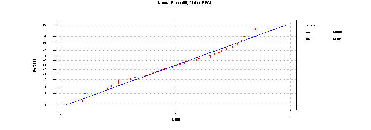
I have used the edit capabilities of Minitab to highlight the points, color them and increase their size so you can see them. Note that there is some systematic deviation from linearity but not a whole lot. In this case this is probably not enough to force us to change our analysis or even enough to merit considering a transformation of the response.

Finally we perform the Kruskal Wallis procedure on the data (STAT > Nonparametrics > Kruskal-Wallis ).


Kruskal-Wallis Test

Kruskal-Wallis Test on Yield   

Name        N    Median    Ave Rank         Z
A           8     3.000        11.1     -1.89
B           8     3.750        21.9      1.87
C           8     4.200        24.4      2.74
D           8     2.850         8.7     -2.72
Overall    32                  16.5

H = 16.50  DF = 3  P = 0.001
H = 16.56  DF = 3  P = 0.001 (adjusted for ties)

With such small p-values it is clear that we reject the null hypothesis of equal variety medians and conclude that the group differ in their true median values.