|
STA
6166 UNIT 2 Section 2 Answers
|
| < | Unit 2 Section 2 Answers |
| To Ag and Env. Answers |
| To Tox and Health Answers |
| To Engineering Answers |
These problems will be computed using SPSS. You can download the SPSS worksheet from here.
1. Do problem 6.63 on page 327. This problem deals with campaign expendatures by gender for individuals running for public office.
a. State the null and alternative hypotheses in
i. plain English and
Null Hypothesis: Female candidates generally spend MORE OR THE SAME in their campaigns for public office as do male candidates.
Alternative Hypothesis: Female candidates generally spend LESS in their campaigns for public office as do male candidates.
ii. statistical terms or symbols.
Let mF represent the AVERAGE expenditure of female candidates and mM represent the AVERAGE expenditure of male candidates. The the hypotheses can be stated as.
Null Hypothesis: mF = mM (actually greater than or equal to but I can't get the correct symbol here)
Alternative Hypothesis: mF < mM
b. Estimate the size of the difference in campaign expenditures for female and male candidates.
We use SPSS to compute the basic statistics for the two groups (ANALYSE>DESCRIPTIVE STATISTICS>DESCRIPTIVES). From this we can compute the estimate of the size of the difference as the difference between the two sample means. In this case, the estimate is mdiff = 245.3-352.0 = -105.7.

c. Is the difference statistically significant at the 0.05 level?
For this we use the two independent samples test option (ANALYSE>COMPARE MEANS>INDEPENDENT SAMPLES T TEST).

SPSS runs both pooled variance and separate variance two independent sampel t-tests. Unfortunately you cannot specify that you wish only a one-sided test and SPSS output above gives you only the two-tailed p-values. Still, from the two-tailed p-value we can get the one-tailed p-value by taking half the two-tailed p-value. Here, the p-value for both tests are less than 0.0005 suggesting that with either test we would reject the null hypothesis that expenditures are equal in favor of the alternative that Females spend less than Males.
d. Is the difference of practical significance?
A difference of $105.7 when the average Female expenditure is $245.3 suggests that Males spend 43% more. This is not only statistically significant, it is practically significant.
2. Using the data from problem 6.63, perform the Wilcoxon rank sum test. Do the t-test and Wilcoxon test give different results?
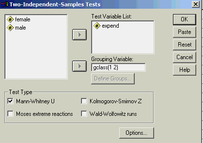
To get SPSS to perform this test we go to the ANALYSE>NONPARAMETRIC TEST>TWO INDEPENDENT SAMPLES > select Mann-Whitney U. It turns out that the Mann-Whitney U test is equivalent to the Man-Whitney-Wilcoxon Rank Sum test. Problem is, the dialog for this test requires stacked data, but the dialog only allows a numeric grouping variable. Thus the gender class variable that has values "m" and "f" will not work. You need to create a new gclass variable with values "1" and "2" and this will work. Such are the pecularities of different packages.


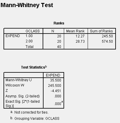
In this case, the alternative hypothesis is that Population 1 (Females) expenditure populations is shifted to the left of the Population 2 (Males) exendature population. The test statistics is the sum of the ranks for Population 1 (Females). The value fo the test statistic is 245 from above. With samples of size 20 in each group, we cannot use Table 5 but must use the Normal Approximation form of the test, page 292. The appropriate value of the z-statistic is given above with the one-tailed significance p-value provided. Since the p-value is much less than the 0.05 type I error rate suggested for the test we conclude that we reject the null hypothesis and conclude the alternative hypothesis that Female expenditures are significantly less than are Male expenditures. This result is the same as that given for the two sample t-tests.
3. What is the 95% confidence interval for the difference between the two means?
The 95% confidence intervals for the difference are given in the table for section c above. Note that the interval assuming separate variances is wider than that created using the pooled variance.
4. How many candidates of each gender would be needed if we wanted to estimate the difference between the average expenditures of the two groups to be within plus or minus $5 with 95% confidence (Hint see page 314).Use the pooled variance estimate from the t-test as if it were the true variance.
SPSS does not do sample size estimation hence we have to use the available information and the equation on page 314 to compute the needed sample size.
The pooled variance estimate is not directly given although we could get it from the standard error of the difference value given above. Instead we will calculate it directly from the equation on page 317, section 1.

The needed sample size is computed for a = 0.05 and signficant difference E=5.

Thus we would need to examine 1004 candidates of each gender if we were to try to estimate the true difference to within $5. Of course this number is quite high and would represent in this case a very significant fraction of the number of individuals in each population. In practice, once the estimated sample size gets much higher than about 5% of the population size there is a correction term that must be applied. This term requires a good estimate of the total number in the population.