From this we would reject the null hypothesis that the two alloys produce beams with equal load capacities in favor of the one-sided alternative that the new alloy is greater than the old alloy. The p-value is < 0.001. We can redo this test assuming a common variance and using a pooled standard deviation estimate to get the following:
Two-sample T for Load

Difference = mu (new) - mu (old)
Estimate for difference:  5.480
95% lower bound for difference: 3.950
T-Test of difference = 0 (vs >): T-Value = 6.21  P-Value = 0.000  DF = 18
Both use Pooled StDev = 1.97
Note that the conclusions of the test do not change, nor is the p-value any different, but the DF for the test is now 18 versus the 13 of the previous problem. The pooled standard deviation estimate is 1.97.
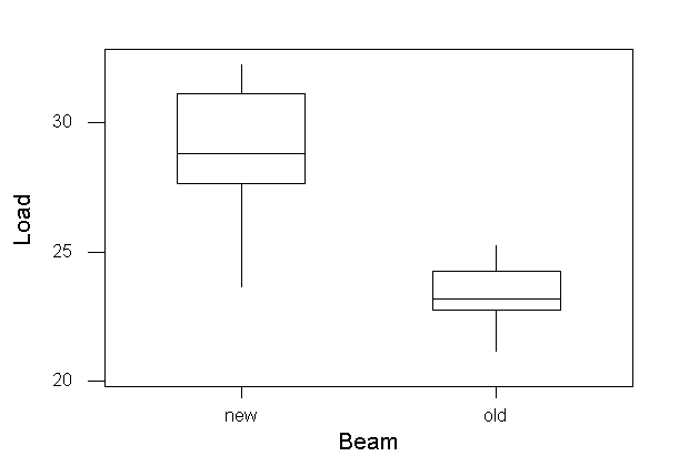
d. Do the condition required for the statistical techniques used in (b) and (c) appear to be satisfied? By this we wonder if the data look sufficiently normal (symmentric, uni-modal). We could look at histograms of the data, but there is very little data here to do this. Box plots don't indicate much to worry about although the distribution do not look exactly symmetric (the median is not in the middle of the inter quartile box..
We could also look at a quantile-quantile plot to determine if the data look sufficiently normal.
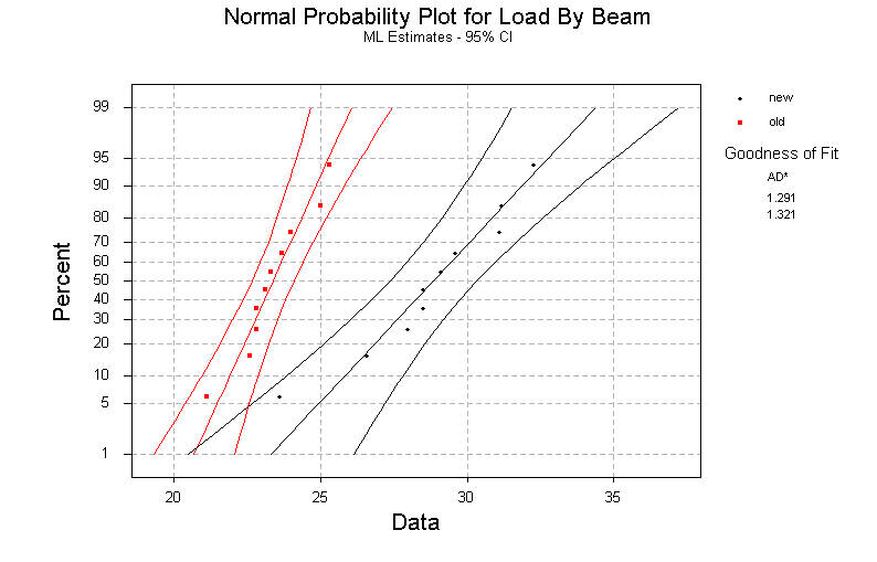
In this plot, if the data are truly normally distributed, they will fall mostly on the straight line. In both cases the data points fall pretty close to the straight line and hence we would conclude that the data are sufficiently normal and that the conditions required for the t-test are met.
e. The beams produced from the new alloy are more expensive thatn the beams produced from the currently used alloy. Thus, the new alloy will be used only if the mean load capacity is at least 5 tons greater than the mean load capacity of the currently used alloy. Based on this information, would you recommend that the company use the new alloy?
To check this, we need to test whether the difference between the two are sufficiently greater than 5 tons. In Minitab, we re-perform the two sample t-test only now we set the significant difference at 5. The results are as follows:
Difference = mu (new) - mu (old)
Estimate for difference:  5.480
95% lower bound for difference: 3.950
T-Test of difference = 5 (vs >): T-Value = 0.54  P-Value = 0.297  DF = 18
Both use Pooled StDev = 1.97
Note that now the null hypothesis of the test is that the difference is 5 versus the alternative that it is greater than 5. The associated p-value is 0.297, suggesting that we cannot reject the null hypothesis that the difference is actually 5 (or less). Since we do not reject the null hypothesis we cannot conclude that the difference in mean load capacity is greater than 5 tons, we would stick with the old alloy for this task.
Note that you may be a little confused with this result. Remember what we are really trying to do is show that the new alloy is 5 tons or greater load capacity than the old alloy. Our test says it is 5 OR LESS but NOT more than 5. Hence we cannot go with the new alloy since there is a high probability the load capacity is actually less than 5 tons and a very low probability that it is greater then 5.
The above computations were run using the full Minitab (on my portable).
The t-test output is from the STAT > BASIC STATISTICS > 2 SAMPLE T.
There is an OPTIONS button on the dialog that allows you put in the difference.
When I attempted to do this in the Student Edition of Minitab, there is no
OPTION button. I didn't notice this before. So, what to do. Well, we know
that subtracting a number from any random variable changes the mean, but does
not change the variance. So in the 'not Stacked' data, create a new "New_New"
column which is the old "NEW" data with 5 subtracted from it. Now
do the two sample t-test of the "New-New" vesus the "OLD"
data to get a t-test that these two groups have the same means. If the original
null hypothesis was that the mean of the NEW beams was 5 tons greater than
that of the OLD beams, then the mean of the NEW-5 group should be the same
as the mean of the OLD group. You should get the correct result.
For the stacked data, create a new column (call it DIFF) with 5 in the rows
for all NEW beam cases and 0 for all OLD beam cases. Now create a second "New_Load"
column with the old response column minus DIFF. Now do the two-sample t-test
(stacked) using this "New_Load" as the response.
2. Using the data from problem 6.37, perform the Wilcoxon rank sum test. Do the t-test and Wilcoxon test give different results?
We will use Minitab. Note first that the Wilcoxon Rank Sum test in Minitab is the same as the Mann-Whitney test (whose name is actually the Mann-Whitney-Wilcoxon Rank Sum test). Next we also note that the Mann-Whitney test does not use "stacked data" but used "unstacked data". Originally I entered the data as stacked data (as I would like you to get into the habit of doing), so I needed to use the Manip>Unstack Columns menu option to get the data into a stacked configuration. The worksheet I have provided to you has already done this. The results of running the Mann-Whitney test is given as:
Mann-Whitney Test and CI: Load_new, Load_old

Load_new   N =  10     Median =      28.800
Load_old   N =  10     Median =      23.200
Point estimate for ETA1-ETA2 is       5.700
95.5 Percent CI for ETA1-ETA2 is (3.801,7.400)
W = 151.0
Test of ETA1 = ETA2  vs  ETA1 > ETA2 is significant at 0.0003
The test is significant at 0.0003 (adjusted for ties)