| General Questions. |
- If two independent random variables, y1 and y2,
are normally distributed with means and variances (m1,
s21) and (m2,s22)
respectively, the difference between the random variables has what
distribution (be specific - give mean and variance).
The difference of two independent normal random variables is itself
a normal random variable having mean equal to the difference of the
two means and variance equal to the sum of the two variances. Hence
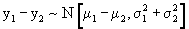
- The sampling distribution of the difference between two sample means
has an approximate normal distribution in large samples with mean
equal to what? If each mean is normal, by the
rule above, the mean for the distribution of the difference of two
sample means should be the difference of the two population means:

- The standard error of the sampling distribution of the difference
between two sample means has what value? Assuming
the population variance for each random variable is known, each sample
mean has corresponding standard error equal to
 .
Hence, by 1 above, we sum the individual variances and then take the
square root to get: .
Hence, by 1 above, we sum the individual variances and then take the
square root to get:  .
This works if the two population variances are assumed known and are
truly different. If they are known to be the same, we can factor the
population variance term out of the sum and even remove it from under
the square root radical sign to get: .
This works if the two population variances are assumed known and are
truly different. If they are known to be the same, we can factor the
population variance term out of the sum and even remove it from under
the square root radical sign to get: 
- The following estimate for the standard error of the difference
between two means is used when what assumption about the two population
variances can be made?
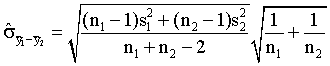 This
estimate is used when we can honestly make the assumption that the
two populations have common variance (or common standard deviations).
The first square root term is our pooled estimate for the value of
this common population standard deviation term. This
estimate is used when we can honestly make the assumption that the
two populations have common variance (or common standard deviations).
The first square root term is our pooled estimate for the value of
this common population standard deviation term.
- What assumption about the two population variances is made when
the following standard error estimate is used?
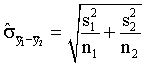 In this case, we are assuming that the two populations
have individual variances (standard deviations) that are NOT equal
to each other. This is referred to as the separate variances estimate
of the standard error of the difference of two sample means.
In this case, we are assuming that the two populations
have individual variances (standard deviations) that are NOT equal
to each other. This is referred to as the separate variances estimate
of the standard error of the difference of two sample means.
- Most of the time in two-population tests, we test the hypothesis
H0: m1-m2
=0. What does it mean to test the hypothesis H0: m1-m2
= D0 where D0 does not equal to zero? The
term D0 refers to the expected difference. When D0
does not equal zero, we are saying that we expect one of the means
to differ from the other mean by this amount on average. So if we
say m1-m2
=10, we are saying that on average we expect the difference between
the means to be 10 units. What we are hoping to do is show (depending
on the alternative hypothesis) that the true difference is different
(less than or greater than) D0.
- Why is the Wilcoxon Rank Sum test use the words "Rank Sum"
in its name? The test statistic used is constructed
as the sum of ranks for the sorted data. In this case, the test statistic
is the sum of the ranks for one of the populations.
- Use Table 5 in the Appendix to find the critical value of the Wilcoxon
rank sum test for independent samples when n1=7 and n2
= 6 and the alternative hypothesis is "Population 1 is shifted
to the right of Population 2" with Type I error probability of
a=0.05. The alternative
hypothesis tells us that we are in Case 1 and that the critical value
will be TU[7,6,a=0.05,one-tailed]=54
- How is the critical value for the Wilcoxon rank sum test found if
one or both of the sample sizes are greater than 10? The
answer is on page 292 in the book. Essentially we revert to a one-sample
z-test where the mean we are comparing the observed rank sum T to
is given by the sample sizes (see the mean value on page 298). The
true variance for the z-statistics depends on the sample sizes as
well as the numbers of tied ranks. Note that the theory behind the
Wilcoxon rank sum test requires that the underlying distributions
are continuous.
- What do we mean when we talk about "Paired Data"? Paired
data refer to data collection (or experimental) conditions where the
measurements for the two "factors" of interest are taken
on the same unit or individual. Because of this, we expect some correlation
or lack of independence between the two measurements, e.g. association
between the paired measurements caused by their being taken on the
same individual. The statistical analyis must take into account this
structural aspect of the sampling. Another way of looking at the paired
data case is as follows. In the two independent sample case we can
conceptually envision randomly assigning study units to treatments.
In the paired data case, the study units are created in pairs, each
pair is defined on one individual. Each individual gets both treatments,
treatments randomly assigned to the paired study units for that individual.
Individuals are hence assumed random.
- Is a two-sample Paired Data t-test equivalent to a one-sample t-test
performed on the differences in values for each sample unit? Why
of course!
- Which of the two tests is for testing the difference in means from
samples of two independent populations? The Wilcoxon Rank Sum Test
or the Wilcoxon Signed Rank Test? So what does the other test? The
Wilcoxon Rank Sum Test is the nonparametric equivalent of the two
independent sample t-test. The Wilcoxon Signed Rank Test is essentially
the equivalent of the one-sample t-test. It is used to for paired
data situations as well as one-sample testing.
- The equation for estimating sample sizes for the two-sided hypothesis
test of differences of means is given by:
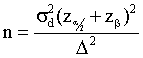 .
Can you define each of the terms in this equation? See
the discussions on pages 315 and 316 in the book. The D
term is defined by how big of a difference between the population
means we feel must occur if the populations are to be declared truly
different. The a
and b relate
to the probabilities of Type I and Type II errors. The sd
is the value of the true standard deviation of the differences. .
Can you define each of the terms in this equation? See
the discussions on pages 315 and 316 in the book. The D
term is defined by how big of a difference between the population
means we feel must occur if the populations are to be declared truly
different. The a
and b relate
to the probabilities of Type I and Type II errors. The sd
is the value of the true standard deviation of the differences.
- Do problem 6.83 as a paired samples t-test and using the Wilcoxon
Signed Rank test, both with a Type I error probability of 0.05. Do
you get different results? Using Excel we can
easily compute the differences, the appropriate t-statistic and compute
the associated t-critical value and p-value.
Sample Analyst_1 Analyst_2 Difference Signed_Rank
          1    31.4    28.1       3.3     5
          2    37.0    37.1      -0.1    -1
          3    44.0    40.6       3.4     6
          4    28.8    27.3       1.5    3.5
          5    59.9    58.4       1.5    3.5
          6    37.6    38.9      -1.3     -2
          Mean Difference=     1.38
          Variance Difference= 3.43
          Standard Deviation=  1.85
          sample size(n)=      6
          t-statistic =        1.83
          t-critical(0.05,5)=  2.02   =tinv(0.10,5)
          p-value=             0.06   =TDIST(D14,5,1)
From this we can determine that the null hypothesis
that Analyst_1 and Analyst_2 read the same cannot be rejected in favor
of the alternative that Analyst_1 reads higher than Analyst_2. For
the Wilcoxon Signed-Rank test we use the computed ranks of the differences
and associated sign as given in the table above. Note that I have
used the average rank for the two tied rankings. Since the differences
were taken as Analyst_1 minus Analyst_2, the alternative hypothesis
is that the median differences should tend to be larger than zero
(Case 1). The test statistic is T-, the absolute value of the sum
of the negative ranks. Here T- = |-3| = 3. The critical value for
the test is obtained from Table 6 for n=5 and a
= 0.05 one-tailed. T-critical = 2. Since T- = 3 > T-critical=2,
we do NOT reject the null hypothesis and conclude that both analysts
are reading similarly. We conclude that both tests lead us to the
same decision.
- Again, using the scenario of problem 6.83 (page 334), how many water
samples would we need if we wanted to be certain that the two Analysts
did not differ by more than 2 ppm with Type I error probability of
0.05 and Power of 0.90 assuming the underlying variance in the differences
were 1.0? Equation on page 316 was used and
programmed into Excel. The following results were obtained.
P(Type I error)=	        	0.05	=C20
P(Type II error)=		    0.10	=C21
Variance of difference=		1.00	=C22
z(alpha) =	    	1.644853	=NORMSINV(0.95)
z(beta)=     		1.281550794 =NORMSINV(0.90)
Delta=	        	2.00	=C25
Expected Sample size =		3	=CEILING(C22*((C23+C24)^2)/(C25^2),1)
From this we conclude that only three samples
are needed. Note that the assumed variances of the differences here
is 1.0 which is less than the 3.43 we observed in the previous section.
If we assumed the variance were 4.0 instead, the needed sample size
would be 9 individuals.
If you have Excel, you can download the simple spreadsheet on which
these calculations were based from here.
Review the Key Formulas on pages 317-318.
|