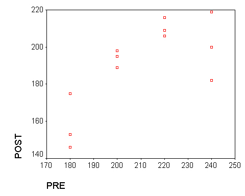
An experiment is run to measure the cholesterol levels on 12 cardiac patients before and after a four-month program of cardiac rehabilitation. For each patient, a reading was taken soon after diagnosis (x) and another was taken after a four-month program of cardiac rehabilitation (y). Three patient were choosen at each of four levels of x. The cholesterol levels obtained were as follows.
pretreatment_level (x)   posttreatment_level (y)
180                               153
180                               146
180                               175
200                               189
200                               198
200                               195
220                               209
220                               206
220                               216
240                               182
240                               200
240                               219
- Plot the sample data in a scatter diagram. By eye, add in the line you think fits the data best.
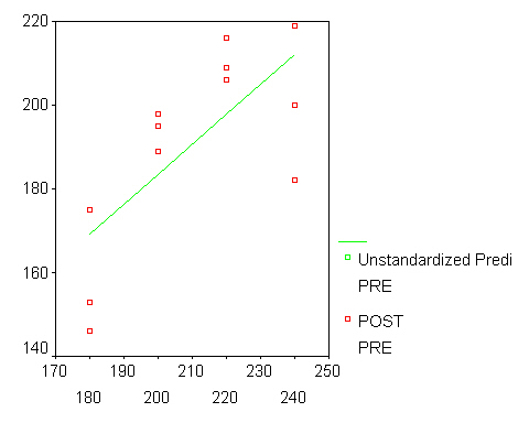
- Estimate the parameters in the model
 and then draw the fitted line onto your scatterplot.
 - Calculate the Analysis of Variance table and test the null hypotheses
of no significant regression. Use

- Location the value of the t statistics for testing
 .
Use .
Show that
.
Use .
Show that  .
. - Calculate the sum of squares due to pure experimental error and lack of fit and write the Anova table. Conduct a test for lack of fit of the linear regression model. Does the linear regression model fit the data well?
- Calculate the variance of
 ,
compute the 95% confidence intervals for .
,
compute the 95% confidence intervals for . - Use the estimated model, predict the values of y when
 =210
and =260.
Find the 95% confidence intervals for
=210
and =260.
Find the 95% confidence intervals for  .
.
We use SPSS to perform this analysis. Enter the data as presented above into the SPSS Data Editor. Before proceeding, type in 210 and 260 in the Pre column. Note that the corresponding values in the Post column are missing. These are the values we will get predictions and confidence bands for.
In the Graphs > Scatter dialog put post on the vertical axis and pre on the horizontal axis. Continue. Select the graph in the View window and go up to Edit > SPSS Chart Object > Open. Now select File > Export Chart. Enter a file name and type (.JPG is good) and Save. This allow you to save a copy of the scatter plot and then place your eye line on the scatter plot (Question 1).
Next we use Analyze> Regression > Linear to bring up the LInear Regression dialog box. Here the Post treatment level is the dependent variable and the Pre treatment level is the independent variable (I prefer response and predictor respectively.) Press the Statistics button to bring up the Statistics dialog box and check off Estimates and Confidence Intervals. Continue. Press the Save button to bring up the Save dialog box. Check Unstandardized Prediction Values; Mean and Individual Prediction Intervals; make sure Confidence Interval is at 95%. Continue. Press OK to compute requested statistics.
This provides the computations needed to answer question 2, 3, 4 and 6 above. Note that the data set, as displayed in the Data Editor now has five (5) more columns. To plot the fitted curve we will plot the pre,post pairs overlayed with the pre,pre_1 pairs. SPSS graphics editing is quite primative so you cannot easily edit the graph options.
For question 5 we need to compute the Pure Error and Lack of Fit statsitics. There are two ways to do this in SPSS, the hard way and the easy way. The easy is truly easy but you don't really see what is being done. Let's do it anyway. Select Analyze > General Linear Model > Univariate and in the dialog place Post as the Dependent variable and Pre and teh covariate. Press Options and in check the Lack of fit box. Continue. OK to get the statistics. The resulting output is below.
The Lack of Fit test is provided for us directly. Note that the Overall regression F-statistic is quite statistically signficant and the Lack of Fit F-statistic is also quite statistically significant (i.e. less than a=0.05). From this we conclude that the slope of the line is not zero but that a linear relationship is not adequate for describing the relationship. We can see the systematic departures from the line and wonder if a quadratic might fit better.
The hard way to get the appropriate sums of squares is to fit the one-way classification ANOVA model following the simple regression. Choose Analyze > General Linear Model > Univariate and in the dialog place Post as the Dependent variable and Pre and the Fixed Factor. Press Model and in the dialog box put pre(F) into the Model: box. Continue. Press OK. In the resulting output we have the Pure Error sums of squares as the Sums of Sqares Error from the ANOVA. We then compute the Lack of Fit sums of squares by subtraction of the Pure Error SS from the Error SS in the Simple Regression model.
Finally, we could compute the predicted value and confidence intervals for the respons at x=210 and 260, but why not let SPSS do it. If you look at the last two lines of the Data Editor you find in the pre_1 column that we predict a post value of 190.6667 for x=210 and a post value of 226.5 for a pre value of 260. Similarly the 95% confidence interval is (lmci_1, umci_1)=(179.8, 201.5) and (199.99, 253.01) respectively. The (lici_1, uici_1) pairs are the prediction interval bounds.