Air with varying concentrations of CO2 is passed over wheat leaves at a temperature of 35°C and uptake of CO2 by the leaves is measured. Three replications are choosen at each of four levels of CO2 . Uptake values (y) for different concentrations (x) are obtained and are as follows:
Concentration(x)   Uptake(y)
75                    .30
75                    .11
75                    .46
100                   .65
100                   .53
100                   .71
125                   .89
125                   .81
125                  1.02
150                  1.20
150                  1.81
150                   .97
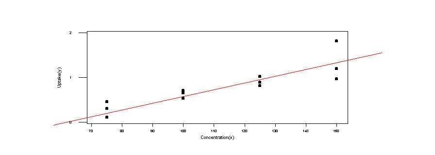
1. Plot the sample data in a scatter diagram. By eye, add in the line you think would fit the data best.
2. Estimate the parameters in the model ![]() and then draw the fitted line onto your scatterplot.
and then draw the fitted line onto your scatterplot.
The regression equation is
Uptake(y) = - 0.736 + 0.0135 Concentration(x)

Predictor        Coef       StDev          T        P
Constant      -0.7357      0.2647      -2.78    0.019
Concentr     0.013547    0.002283       5.93    0.000

The variance of the residual terms is estimated by the mean square error to be 0.0489.
3. Calculate the Analysis of Variance table and test the null hypotheses
of no significant regression. Use![]()
Analysis of Variance

Source            DF          SS          MS         F        P
Regression         1      1.7204      1.7204     35.20    0.000
Residual Error    10      0.4887      0.0489
Total             11      2.2092
Since the p-value associated with the F-statistic is less than the specified Type I Error rate, we conclude that the regression is statistically significant. By this we conclude that the slope of the regression line is not equal to zero.
4. Calculate the value of the t statistic for testing ![]() .
Use
.
Use ![]() .
Show that
.
Show that ![]() .
.
From the table given in question 1 above, we find that the t-ststistic for testing that the slope is equal to zero is t=5.93 with associated p-value<0.0005. Note that (5.93)2 = 35.165 which rounds to F=35.20. Note that with more significant digits in the computation of both F and t, the values would be exactly equal. This is always the case for 1 degree of freedom F-tests.
5. Calculate the sum of squares due to pure experimental error and lack of fit and write the associated ANOVA table. Conduct a test for lack of fit of the linear regression model. Does the linear regression model fit the data well.
MINITAB will not directly compute the expanded ANOVA table for the lack of fit test, but we can get it to make the calculations for us. First, we need to realize that the Pure Experimental Error term is simply the error term from a one-way analysis of variance run on the data where we set Concentration as a classification term rather than a quantitative term. So, run the one-way ANOVA using STAT > ANOVA > One Way > Response: 'Uptake' Factor: 'Concentration'; We get the following ANOVA table.
Analysis of Variance for Uptake(y
Source     DF        SS        MS        F        P
Concentr    3    1.7316    0.5772     9.67    0.005
Error       8    0.4775    0.0597
Total      11    2.2092
Now, we have our estimate for the Pure Error Sums of Squares at 0.4775 with degrees of freedom 8. The Lack of Fit Sums of Squares is the difference between the Concentration sums of squares from the ANOVA model and the Concentration sums of squrares from the Regression, i.e. 1.7316 - 1.7204 = 0.0112. Similarly the degrees of freedom is 3-1 = 2. The final analysis of variance table is
Analysis of Variance

Source            DF          SS          MS         F        P
Regression         1      1.7204      1.7204     35.20    0.000
Residual Error    10      0.4887      0.0489
  Lack of Fit       2       0.0112      0.0056    0.094   0.9114
  Pure Error        8       0.4775      0.0597
Total             11      2.2092
From the F-statistic for the lack of fit test we conclude that there is little chance that the linear model is not adequate, ie. the linear model is an adequate description of the relationship between concentration and uptake.
6. Calculate the variance of both![]() and compute the associated 95% confidence intervals.
and compute the associated 95% confidence intervals.
From the table of estimated values for b0 and b1 we have the estimated standard deviations. The variance of the estimates is simply the square of these terms. We then use these terms to compute the 95% confidence intervals using the value of t(10,0.025) = 2.228.
Predictor        Coef       StDev       Var        Lower 95% Bound   Upper 95% Bound
Constant      -0.7357      0.2647       0.07007    -1.325             -0.1459
Concentr     0.013547    0.002283       5.212E-6   0.00846             0.01863
7. Using the estimated model, predict the values of y when ![]() =90
and
=90
and ![]() =150.
Find the 95% prediction intervals for
=150.
Find the 95% prediction intervals for ![]() .
.
There are two ways to get MINITAB to compute these values. First is to use the Options button on the Regression dialog box and type in 90 in the "Prediction intervals for new observations" box. Then run the regression and you will get the folowing output. You have to rerun the regression after replacing the 90 with 150 in the "Prediction intervals..." box to get the second output.
Predicted Values


     Fit  StDev Fit         95.0% CI             95.0% PI
  0.4835     0.0819   (  0.3010,  0.6661)  ( -0.0418,  1.0089)
Predicted Values


     Fit  StDev Fit         95.0% CI             95.0% PI
  1.2963     0.1068   (  1.0584,  1.5343)  (  0.7493,  1.8434
A second approach is to add two points to the data set with concentration equal to 90 and 150 and the associated uptake as missing.
Concentration(x)	Uptake(y)
75	0.30
75	0.11
75	0.46
100	0.65
100	0.53
100	0.71
125	0.89
125	0.81
125	1.02
150	1.20
150	1.81
150	0.97
90	*
150	*
Then in the dialog box for the Options for regression insert 'Concentration' in the "Prediction Intervals for new obsrevations:" box then check Fits, SDs of fits, Confidence limits and Prediction limits and make sure the Confidence level is 95. You will then get the following output, with CLIM6 and CLIM7 as the upper and lower confidence limits and PLIM6 and PLIM7 the upper and lower bounds for the prediction limits.
FITS6	PFIT6	PSDF6	     CLIM6	  CLIM7	  PLIM6	    PLIM7
0.28033	0.28033	0.106789	0.04239	0.51827	-0.266710	0.82738
0.28033	0.28033	0.106789	0.04239	0.51827	-0.266710	0.82738
0.28033	0.28033	0.106789	0.04239	0.51827	-0.266710	0.82738
0.61900	0.61900	0.069910	0.46323	0.77477	 0.102372	1.13563
0.61900	0.61900	0.069910	0.46323	0.77477	 0.102372	1.13563
0.61900	0.61900	0.069910	0.46323	0.77477	 0.102372	1.13563
0.95767	0.95767	0.069910	0.80190	1.11344	 0.441039	1.47429
0.95767	0.95767	0.069910	0.80190	1.11344	 0.441039	1.47429
0.95767	0.95767	0.069910	0.80190	1.11344	 0.441039	1.47429
1.29633	1.29633	0.106789	1.05839	1.53427	 0.749290	1.84338
1.29633	1.29633	0.106789	1.05839	1.53427	 0.749290	1.84338
1.29633	1.29633	0.106789	1.05839	1.53427	 0.749290	1.84338
0.48353	0.48353	0.081927	0.30099	0.66608	-0.041788	1.00885
1.29633	1.29633	0.106789	1.05839	1.53427	 0.749290	1.84338