Maple Files for Computation of Puiseux Expansions for Singular Points of Algebraic Curves

Single Maple File

2,2 talk — best viewed in Classic Worksheet mode; double points of real quintic curves.

4th Degree

Multiplicity 2

• 

  2,2

  Maple worksheet, Word document

Multiplicity 3

• 

  2,1,1

  Maple worksheet, Word document

5th Degree

Multiplicity 2

• 

  2,2

  Maple worksheet, Word document

Multiplicity 3

• 

  2,1,1

  Maple worksheet, Word document

• 

  2,2,1

  Maple worksheet, Word document

• 

  3,1,1

  Maple worksheet, Word document

Multiplicity 4

• 

  2,1,1,1

  • Three factors the same: Maple worksheet, Word document
  • Two factors the same: Maple worksheet, Word document

• 

  3/2,1,1

  Maple worksheet, Word document

6th Degree

Multiplicity 2

• 

  3,3

  Maple worksheet, Word document

Multiplicity 3

• 

  2,2,2

  • Two factors the same: Maple worksheet, Word document
  • Three factors the same: Maple worksheet, Word document

• 

  2,2,1

  Maple worksheet, Word document

Multiplicity 4

• 

  2,1,1,1

  Maple worksheet, Word document

• 

  3/2,1,1

  Maple worksheet, Word document

• 

  3/2,3/2

  Maple worksheet, Word document

• 

  2,2,1,1

  • All on 1: Maple worksheet, Word document
  • All on 2: Maple worksheet, Word document
  • Everything between: Maple worksheet, Word document

Multiplicity 5

• 

  2,1,1,1,1

  Maple worksheet, Word document

• 

  3/2,1,1,1

  Maple worksheet, Word document

• 

  4/3,1,1

  Maple worksheet, Word document

References from Maple Worksheets

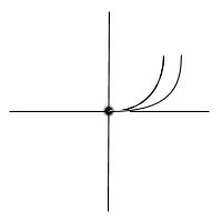
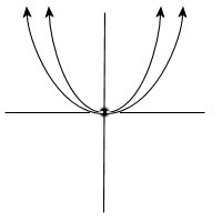
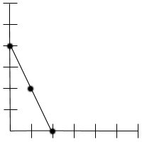
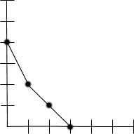
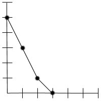
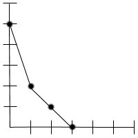
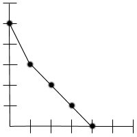
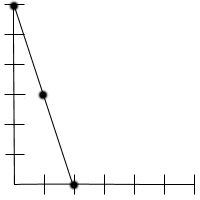
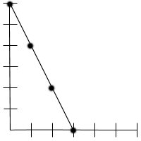
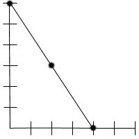
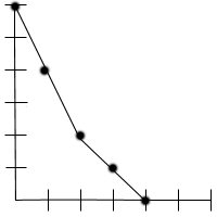
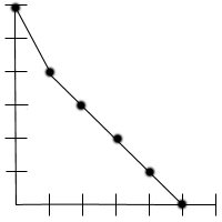
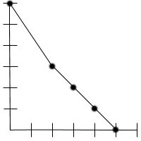
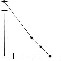
1. First we define the polynomial based on the Newton polygon. Each point on the polygon represents a term in the polynomial, where the vertical coordinate is equal to the x-exponent and the horizontal coordinate is equal to the y-exponent of the term. The coefficients are literal to include the entire family represented by the polygon.
2. The Puiseux algorithm computes terms until the jets differ. When the highest power of the coefficients of x in the jet is a fractional power, we have multiple roots, so we can make the jets the same by setting the coefficient of that term equal to zero. This forces Puiseux to calculate the next term, which has a higher power, and the splitting will be at that term.
3. We reevaluate the polynomial where the coefficients of the highest power term in the Puiseux jet of the previous expansion are equal to zero. This requires that, when the expression is set to zero, we solve for a variable in order to make a substitution, so there will often be a solving step.
4. As in [2], we want to make the jets the same. When the highest power of the coefficients of x in the jet is a whole power, we have multiple roots represented in a RootOf() expression. Therefore, we take the discriminant of the polynomial in _Z and set it equal to zero so that the coefficients in the highest power terms of the jets will be the same.
5. Once the polynomial factors, it is apparent that the curve is reducible. At this point, the proof is complete. When it does not factor, the step is not shown, but we do attempt to factor the polynomial at every step.
6. In this case, the polynomial does not factor, but we see from the Puiseux expansion that all of the jets have completely split.
7. Because the numerator factors, we must consider both cases where the numerator is equal to zero.
8. Using a T in the Puiseux argument will parameterize the output, making it easier for Maple to compute. The Puiseux function can give unnecessarily large answers. Reading the following code into Maple before using the Puiseux function will help prevent one, but not all, causes of these large answers by reducing some unnecessary expanding.