DiffEq 2 Mathematica crash course
Numbers
Numbers will be represented symbolically when possible
![]()
![]()
A floating point approximation can be computed using the N function.
![]()

You can go to arbitrary precision
![]()
![]()
![]()

You can apply the N function after an operation
![]()
![]()
Arithmetic
Addition, subtraction, multiplication, and division are defined as usual. Multiplication is implicit for symbols separated by whitespace
![]()
![]()
![]()

Warning: a missing whitespace can cause a subtle error.
![]()
![]()
![]()
![]()
This is a common beginner’s mistake. If you look carefully you can see that u v and uv are rendered in different fonts.
To be on the safe side, you can always use the “*” operator for multiplication
![]()
![]()
Math functions
The usual mathematical functions are defined. All built-in function names are capitalized. Function arguments are put in square brackets not parentheses.
![]()
![]()
![]()
![]()
![]()
![]()
Warning: See what happens if you forget to capitalize:
![]()
![]()
This error can be hard to detect. Notice that the word “sin” is rendered in a colored font (indicating that it hasn’t been defined yet). Notice also that Mathematica can’t recognize that sin[Pi] is zero, because the “sin” function (as opposed to the “Sin” function) isn’t defined.
Warning: See what happens if you use parentheses instead of square brackets:
![]()
![]()
All of your familiar friends are available as built-in functions:


Here are some new friends you’ll meet later this semester
![]()
![]()
![]()
![]()
Plotting functions of one variable
Plot a function
![]()
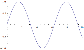
Plot two functions together
![]()
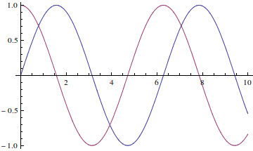
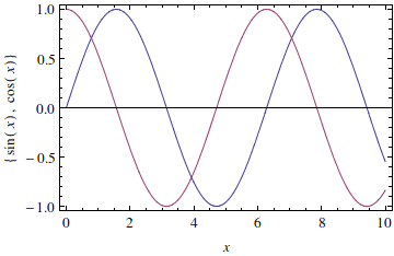
Make the plot a little prettier. See the documentation for lots of plotting options.

Defining your own functions
You can define your own functions very easily, as long as you pay attention to one small detail: put an underscore after the variable name.
The following defines a function f of a variable x
![]()

When I evaluate f at different arguments it does the right thing
![]()

Warning: the following defines the value of a function g at a specific argument value x.
![]()

When I try to evaluate g at different arguments it doesn’t know how to compute g except at the specific input x. This is probably not what you want.
![]()

Most of the time you’ll want to put an underscore after argument names when defining functions. See the documentation for further information about function arguments; if you want to get fancy you can define optional arguments, handle different argument types differently, set default values, and other neat tricks, but you’ll not need to do that for any problems in this course.
You can also make multivariable functions
![]()
![]()
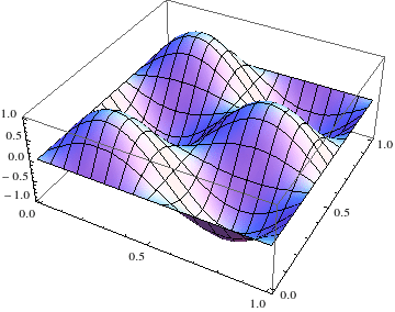
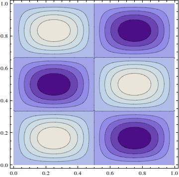
and you can plot them in several ways:
![]()
![]()
Lists
I’ve been using lists enclosed in curly braces already. Here’s a little more information on them.
You can nest lists inside of lists:
![]()
![]()
You can access list elements by index
![]()
![]()
You can access elements by index relative to the end
![]()
![]()
Ranges of indices are specified with the double semicolon operator (analogous to Matlab’s colon operator)
![]()
![]()
You can index into more than one level
![]()
![]()
You can “flatten” a structured list into a simple list
![]()
![]()
Many operations “thread” over lists
![]()
![]()
![]()
![]()
![]()
![]()
Table: generating lists from a formula for the elements
We’ll often be given a formula for the i-th entry in a list, such as 
![]()
![]()
We can make 2D tables by iterating over two indices. The first index is for the rows, the second for the columns
![]()
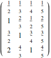
Tables don’t have to be rectangular
![]()

Vectors
A vector is just a list
![]()
![]()
Access vector elements just like you do with a list: use x[[1]] to access the first element of a vector.
![]()
![]()
![]()
![]()
Vector addition and subtraction are done using the + and - operators
![]()
![]()
![]()
![]()
Dot product is done with the period (“.”) operator or the Dot function
![]()
![]()
![]()
![]()
The 3D cross product is done with the Cross function
![]()
![]()
What does the multiplication operator do?
![]()
![]()
How about the division operator?
![]()
![]()
![]()
![]()
![]()
![]()
Warning: Mathematica makes no distinction between row vectors and column vectors. This is a significant difference from MATLAB, which carefully distinguishes between the two. It’s convenient when you don’t care about the difference, but can sometimes cause trouble.
Matrices
Matrices are just rectangular lists.
![]()

![]()

The usual matrix-matrix operations are defined:
![]()

![]()

Matrix-matrix multiplication uses the dot (“period”, “.”) operator, just like the dot product
![]()

Warning: be sure to use the dot, not * or implicit multiplication!
![]()

![]()

Matrix-vector multiplication also uses the dot operator
![]()
![]()
![]()
![]()
Warning: don’t forget to use the dot!
![]()

Linear algebra
You can solve A x=b
Choose a vector for the answer x
![]()
![]()
Multiply our answer by A to produce a RHS
![]()
![]()
Solve the system using the LinearSolve function
![]()
![]()
You can also solve the system numerically. This will be more efficient for large systems.
![]()
![]()
You can compute the inverse
![]()

and then use it to solve the system: ![]()
![]()
![]()
I’ll explain in a few days why that’s usually not a good idea. For now, I’ll just tell you: you should always solve linear systems of equations using LinearSolve rather than multiplying by an inverse. And never, never, never use Cramer’s Rule.
Finding eigenvalues and eigenvectors
You can find eigenvalues and eigenvectors symbolically for simple enough matrices.
![]()
![]()
![]()

The Eigensystem function finds both together.
![]()

You’ll soon learn that it’s generally impossible to find exact eigenvalues and eigenvectors for matrices above size four-by-four, and even for three-by-three the exact eigenvalues might be messy to compute.
![]()

![]()

However, there are efficient algorithms for computing approximate eigenvalues numerically. Just give a floating point matrix to the Eigenvalues function and a good algorithm will be used.
![]()
![]()
(Unfortunately, at the level of this course I can’t explain to you the wonderfully ingenious algorithms used to compute approximate eigenvalues. Practical eigenvalue algorithms are nothing like the methods you’ll learn soon for simple hand calculations. But you can trust that Mathematica, MATLAB, and similar programs have good “black box” algorithms for finding approximate eigenvalues for matrices of dimension up to a few thousand rows.)
Polynomials
![]()
![]()
You can factor any polynomial that has integer roots
![]()
![]()
![]()
![]()
You can solve polynomial equations exactly (up to degree four, and in special cases higher degree):
![]()
![]()
![]()

Most polynomials of degree 5 or above can’t be solved exactly
![]()
![]()
![]()

In such cases, use NSolve to find a numerical solution
![]()
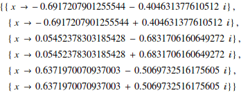
The Solve function will find complex roots:
![]()
![]()
Manipulating expressions
![]()
![]()
![]()

![]()

![]()
![]()
Calculus
![]()

Limits
![]()
![]()
![]()
![]()
Derivatives
![]()

![]()

![]()

Compute derivatives of ![]() through order 10
through order 10
![]()

Partial derivatives
![]()
![]()
Partial wrt x
![]()
![]()
Partial wrt y
![]()
![]()
Second partial wrt x
![]()
![]()
Laplacian: ![]()
![]()
![]()
Indefinite integrals
Mathematica can do elementary integrals
![]()
![]()
![]()
![]()
Some may return results in terms of functions that probably aren’t familiar to you:
![]()

Some can’t be done exactly at all in terms of any known functions. If the result returned is a integral, that means Mathematica’s integration algorithms weren’t able to compute it.
![]()
![]()
Definite integrals
In this course we will be doing very many definite integrals (for reasons that will become clear later). So get used to working with the Integrate function!
You can do simple definite integrals easily with Mathematica
![]()
![]()
![]()
![]()
![]()

Complicated integrals might return unfamiliar functions
![]()

![]()
![]()
You can do improper integrals
![]()
![]()
Some integrals are too hard even for Mathematica. If the result is returned as an “undone” integral, that means Mathematica couldn’t find an exact result with its algorithms.
![]()
![]()
In such cases, numerical integration can be used.
![]()
![]()
Finally, if you try to integrate a function that hasn’t yet been defined, Mathematica won’t know what to do and will simply return an “undone” integral.
![]()
![]()
![]()
Laplace transforms
![]()
![]()
![]()

![]()
![]()
![]()
![]()
![]()
![]()
Differential equations
General soln
![]()
![]()
Initial value problem
![]()
![]()
Boundary value problem
![]()

The result is returned as a substitution rule. The expression

is a rule that, when executed, replaces the symbol y(t) by the stuff after the arrow.
Notice also that the result is a list of substitution rules. This is because, in general, differential equations can have more than one solution.
Digression: substitution rules
Here's a simple example or using a subst rule:
![]()
![]()
Here’s a more complicated example:
![]()
![]()
![]()
![]()
Working with DSolve solutions
Capture the result of DSolve into a variable. Select the first list element (since in this course we’ll always have unique solutions).

![]()
Now create a function using the symbol y(t) acted upon by the rule:
![]()
![]()
Warning: I always use different names to distinguish between the symbolic unknown y(t) and the solution ySoln(t). The reason is that once you define a value for y(t), then if you use that symbol in another call to DSolve Mathematica will evaluate all expressions involving it, including the equality tests such as y[0]==1. That evaluation will return True or False depending on the equation and the value of y[t]. DSolve won’t know what to do with that input, and will give you a strange error message. About all you can do at that point is restart Mathematica.
Long story short: never do something like
y[t_]=y[t] /. solnRule. Always use a variable name for your evaluatable solution function different from the name you used for the unknown.
Warning #2: Be very, very careful to use double-equals operators (“==”) instead of single-equals (“=”) in defining your equations. Double equals tests for equality, single equals does an assignment (if you know C, C++, Python, Java, etc this will be familiar). If you use single equals the input to DSolve will confuse it. I know of no way to recover from this error except to restart Mathematica.